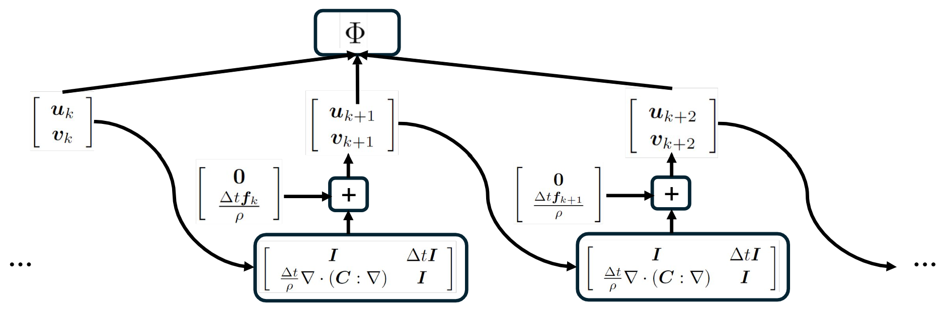
Under time discretization, the FWI problem constrained by the wave equation $$\rho\frac{\partial^2 \mathbf{u}}{\partial t^2}-\nabla\cdot(\mathbf{C}:\nabla\mathbf{u}) = \mathbf{f}$$ can be seen as training a simplest recurrent neural network (RNN) with linear activation. See the following diagram:
Following the backpropagation algorithm, we can obtain the gradient of the objective function $\Phi$ with respect to the model parameters $\rho$ and $\mathbf{C}$. The path for backpropagation is shown in red in the following diagram:
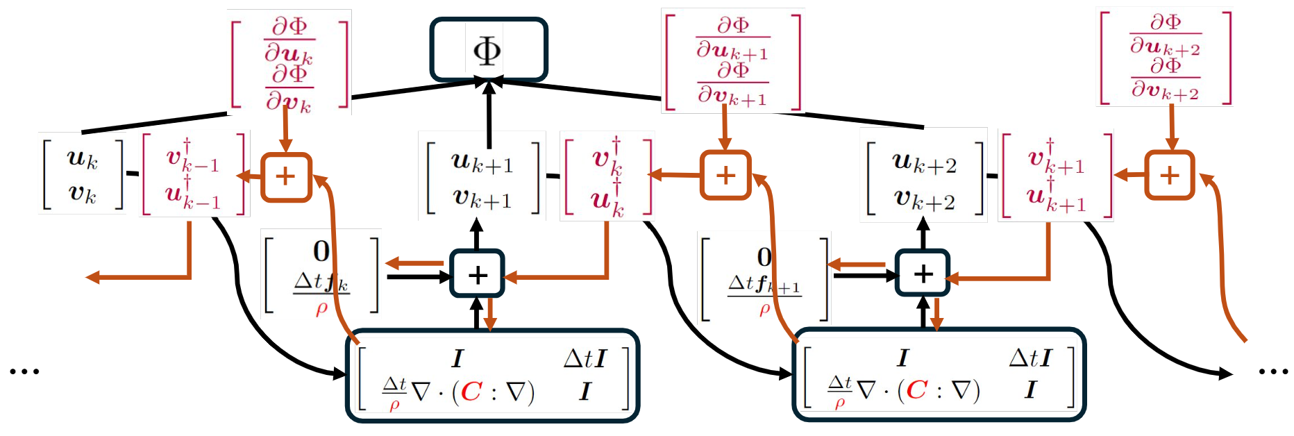
It can be verified that as $\Delta t\rightarrow 0$, the gradient calculated by backpropagation is identical to the sensitivity kernel calculated using the adjoint method in FWI literature, e.g., Tromp, Tape & Liu (2005). This indicates that although derived from different perspectives, the adjoint method in FWI is equivalent to the backpropagation algorithm in deep learning.
To further illustrate this idea, I implement the RNN that represents the wave equation using PyTorch. Then, I use the auto-differentiation and backpropagation functionality of PyTorch to calculate the gradient. As can be seen below, the gradient given by PyTorch is identical to that shown in Tromp, Tape & Liu (2005) based on the adjoint method. The code was run on Google Colab.
import torch
import numpy as np
import torch.nn as nn
import matplotlib.pyplot as plt
from matplotlib import rc
from matplotlib.animation import FuncAnimation
from IPython.display import HTML # so that it works on Colab
Now we define an RNN model representing the wave equation. The spacial gradients are approximated using the first-order staggered-grid finite-difference velocity-stress scheme for simplicity, but any other schemes can be used as well. Same as Section 7.2.1 of Tromp, Tape & Liu (2005), we only consider the SH (scale) wave here.
class Wave2d_SH_fd(nn.Module):
def __init__(self, par, model):
  super(Wave2d_SH_fd, self).__init__()
  self.dt = par.dt; self.dx = par.dx; self.dz = par.dz
  self.left_bc = par.left_bc; self.right_bc = par.right_bc
  self.bottom_bc = par.bottom_bc; self.top_bc = par.top_bc
  self.Nt = par.Nt
  self.save_every = par.save_every
  self.f0 = par.f0
  self.save_type = par.save_type
  self.rho_vtx = nn.Parameter(torch.from_numpy(model.rho_vtx), requires_grad=False)
  self.mu_facex = nn.Parameter(torch.from_numpy(model.mu_facex), requires_grad=True)
  self.mu_facez = nn.Parameter(torch.from_numpy(model.mu_facez), requires_grad=False)

def compute_dv_SH(self, vy, tauxy, tauyz, fy):
  # compute dv/dt
  dvydt = torch.zeros_like(vy)
  dvydt[1:-1,:] += (tauxy[1:,:] - tauxy[:-1,:]) / self.dx
  dvydt[:,1:-1] += (tauyz[:,1:] - tauyz[:,:-1]) / self.dz
  # 1st-order paraxial (absorbing)
  if (self.left_bc == 0):
    dvydt[0,:] += (tauxy[0,:] - torch.sqrt(self.rho_vtx[0,:] * self.mu_facex[0,:])
                    * vy[0,:]) / self.dx * 2.0
  if (self.right_bc == 0):
    dvydt[-1,:] += (-torch.sqrt(self.rho_vtx[-1,:] * self.mu_facex[-1,:]) * vy[-1,:]
                    -tauxy[-1,:]) / self.dx * 2.0
  if (self.bottom_bc == 0):
    dvydt[:,0] += (tauyz[:,0] - torch.sqrt(self.rho_vtx[:,0] * self.mu_facez[:,0])
                    * vy[:,0]) / self.dz * 2.0
  if (self.top_bc == 0):
    dvydt[:,-1] += (-torch.sqrt(self.rho_vtx[:,-1] * self.mu_facez[:,-1]) * vy[:,-1]
                    -tauyz[:,-1]) / self.dz * 2.0
  # zero traction
  if (self.left_bc == 2):
    dvydt[0,:] += tauxy[0,:] / self.dx * 2.0
  if (self.right_bc == 2):
    dvydt[-1,:] += -tauxy[-1,:] / self.dx * 2.0
  if (self.bottom_bc == 2):
    dvydt[:,0] += tauyz[:,0] / self.dz * 2.0
  if (self.top_bc == 2):
    dvydt[:,-1] += -tauyz[:,-1] / self.dz * 2.0
  dvydt = (dvydt + fy) / self.rho_vtx
  # zero displacement
  if (self.left_bc == 1):
    dvydt[0,:] = 0.0
  if (self.right_bc == 1):
    dvydt[-1,:] = 0.0
  if (self.bottom_bc == 1):
    dvydt[:,0] = 0.0
  if (self.top_bc == 1):
    dvydt[:,-1] = 0.0
  return dvydt

def compute_dtau_SH(self, vy):
  # compute dtau/dt
  dtauxydt = (vy[1:,:] - vy[:-1,:]) / self.dx * self.mu_facex
  dtauyzdt = (vy[:,1:] - vy[:,:-1]) / self.dz * self.mu_facez
  #dtauxydt[:,:] *= self.mu_facex[:,:]
  #dtauyzdt[:,:] *= self.mu_facez[:,:]
  return dtauxydt, dtauyzdt

def update_SH(self, vy, tauxy, tauyz, fy):
  # update v, tau
  dvydt = self.compute_dv_SH(vy, tauxy, tauyz, fy)
  vy = vy + dvydt * self.dt
  dtauxydt, dtauyzdt = self.compute_dtau_SH(vy)
  tauxy = tauxy + dtauxydt * self.dt
  tauyz = tauyz + dtauyzdt * self.dt
  return vy, tauxy, tauyz

def forward(self, x):
  vy = x[0,...]
  tauxy = x[1,:-1,:]
  tauyz = x[2,:,:-1]
  fy0 = x[3,...]
  if (self.save_type == 'seismogram'):
    g0 = x[4,...]
  Nsave = len(range(0, self.Nt, self.save_every))
  if (self.save_type == 'snapshot'):
    vy_save = torch.zeros(Nsave, x.shape[1], x.shape[2], dtype=torch.float)
  elif (self.save_type == 'seismogram'):
    vy_save = torch.zeros(Nsave, dtype=torch.float)
  fy = torch.zeros(x.shape[1], x.shape[2], dtype=torch.float)
  t = -1.2 / self.f0
  CALC_STF = True
  # main for loop for time stepping
  for i in range(0, self.Nt):
    if CALC_STF:
      if (t < (3.0 / self.f0)):
        sourcetime=np.exp(-np.pi*np.pi*self.f0*self.f0*t*t)
        fy = fy0 * sourcetime
      else:
        fy[:,:] = 0.0
        CALC_STF = False
    vy, tauxy, tauyz = self.update_SH(vy, tauxy, tauyz, fy)
    if ((i % self.save_every) == 0):
      if (self.save_type == 'snapshot'):
        vy_save[i//self.save_every,:,:] = vy
      elif (self.save_type == 'seismogram'):
        vy_save[i//self.save_every] = torch.sum(vy * g0)
    t = t + self.dt
  return vy_save
Next we define a functional to measure the travel-time shift between synthetics and data. Note that since the $\mathrm{argmax}$ term causes trouble for auto-differentiation, we need to manually tell PyTorch how to calculate the derivative, which is the so-called adjoint source in FWI literature. This derivation of the travel-time adjoint source dates back to Dahlen, Hung & Nolet (2000).
class TravelTimeMisfit(torch.autograd.Function):
@staticmethod
def forward(ctx, syn, dat, win, dt, nshift_max):
  syn_w = syn * win
  dat_w = dat * win
  dat_w_shift = torch.cat((dat_w[nshift_max:], torch.zeros(nshift_max, dtype=float)))
  cc_max = 0.0
  tshift = -nshift_max * dt
  for ishift in range(-nshift_max, nshift_max+1):
    cc = torch.sum(dat_w_shift * syn_w) / torch.sqrt(torch.sum(dat_w_shift * dat_w_shift) * torch.sum(syn_w * syn_w))
    if cc > cc_max:
      cc_max = cc
      tshift = ishift * dt
    dat_w_shift = torch.cat((torch.zeros(1, dtype=float), dat_w_shift[:-1]))

  ctx.save_for_backward(syn_w, dt, tshift)
  return tshift

@staticmethod
def backward(ctx, grad_output):
  syn_w, dt, tshift = ctx.saved_tensors
  syn_w_d = torch.cat((torch.zeros(1, dtype=float), syn_w[1:] - syn_w[:-1])) / dt
  syn_w_dd = torch.cat((syn_w_d[1:] - syn_w_d[:-1], torch.zeros(1, dtype=float))) / dt
  Nr = torch.sum(syn_w_dd * syn_w) * dt
  return syn_w_d * dt *tshift / Nr, None, None, None, None
We define a class that can conveniently pass parameters to the model.
class dict2class():
def __init__(self, my_dict):
  for key in my_dict:
    setattr(self, key, my_dict[key])
Then, we define the parameters for the solver (computational domain, grid spacing, time discretization, velocity model, etc.), and instantiate the forward model.
Nex = 660
Nez = 330
xmin = -100000.0
xmax = 100000.0
zmin = -50000.0
zmax = 50000.0
Na = 4
dx = (xmax - xmin) / Nex
dz = (zmax - zmin) / Nez
a = Na * max(dx, dz)
CFL = 0.4 / np.sqrt(2.0)
vy = np.zeros(shape=(Nex+1, Nez+1), dtype=float)
tauxy = np.zeros(shape=(Nex+1, Nez+1), dtype=float) # real shape is (Nex, Nez+1), pad to make shape uniform
tauyz = np.zeros(shape=(Nex+1, Nez+1), dtype=float) # real shape is (Nex+1, Nez), pad to make shape uniform
x, z = np.meshgrid(np.linspace(xmin, xmax, Nex*2+1), np.linspace(zmin, zmax, Nez*2+1), indexing='ij')

def get_model(x, z):
  rho_arr = np.ones_like(x) * 2600.0
  mu_arr = np.ones_like(x) * 2.66e10
  ## change wave speed, upper-right 30% faster, lower-left 30% slower
  # (x1, z1) = (400.0, 400.0)
  # r1 = 100.0
  # mu_arr += np.exp(-((x-x1)**2+(z-z1)**2)/(r1**2)) * 0.7
  # (x2, z2) = (200.0, 200.0)
  # r2 = 100.0
  # mu_arr += np.exp(-((x-x2)**2+(z-z2)**2)/(r2**2)) * (-0.5)
  return rho_arr, mu_arr

def get_force(x, z, xs, zs):
  r = np.sqrt((x-xs)**2 + (z-zs)**2)
  f = np.where(r<=a, (1-(r/a)**2)**3, 0.0)
  return f / np.sum(f)

rho_arr, mu_arr = get_model(x, z)
f0 = 0.03* np.amin(np.sqrt(mu_arr / rho_arr)) / max(dx, dz) # Hertz
dt = CFL * min(dx, dz) / np.amax(np.sqrt(mu_arr / rho_arr))
par_dict = {'dx':dx, 'dz':dz, 'Nex':Nex, 'Nez':Nez, 'dt':dt, 'left_bc':0, 'right_bc':0, 'bottom_bc':0, 'top_bc':0,
#            'Nt':1500, 'f0':f0, 'save_every':100, 'save_type':'snapshot'} # output snapshots
            'Nt':1600, 'f0':f0, 'save_every':5, 'save_type':'seismogram'} # output seismogram
par = dict2class(par_dict)
model_dict = {'rho_vtx':rho_arr[::2,::2], 'mu_facex':mu_arr[1::2,::2], 'mu_facez':mu_arr[::2,1::2]}
model = dict2class(model_dict)

f = get_force(x, z, -50000.0, 0.0) # source
fy = f[::2,::2]
g = get_force(x, z, 50000.0, 0.0) # receiver
gy = g[::2,::2]
inp = torch.from_numpy(np.array([vy, tauxy, tauyz, fy, gy], dtype=float)) # input to the solver
solver = Wave2d_SH_fd(par=par, model=model)
Now we run the forward solver, and perform the measurement between the synthetic and the "data", which is simply a time-shifted version of the synthetics.
syn = solver(inp)
dat = torch.cat((syn[2:], torch.zeros(2, dtype=float)))
win = torch.ones_like(syn, dtype=float)
tt_misfit = TravelTimeMisfit.apply
loss = tt_misfit(syn, dat, win, torch.from_numpy(np.array([par.dt])), 5) # the last argument defines the maximum allowed time shift
print(loss.item())
Launch the backpropagation. Here we do not need to be bothered by the details of adjoint simulation, kernel calculation, etc. PyTorch takes care of everything.
loss.backward()
Plot the calculated gradient, which is identical to Figure 4(a) of Tromp, Tape & Liu (2005).
mu_facex_grad = solver.mu_facex.grad.numpy()
kernel = mu_facex_grad * model.mu_facex
fig, ax = plt.subplots()
ax.set_aspect('equal')
norm = abs(kernel).max()
p = ax.pcolormesh(x[1::2,::2].T, z[1::2,::2].T, kernel.T, vmin=-0.5*norm, vmax=0.5*norm, cmap='bwr_r')
fig.colorbar(p, location='bottom')
plt.savefig("kernel_pytorch.png", bbox_inches='tight')
The output figure:
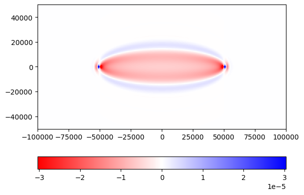
Remark: The program uses a lot of memory. In fact, the program almost consumes all the memory available on Google Colab. This is because PyTorch saves the entire forward wavefield in order to run backpropagation. In FWI, we are usually much smarter on memory usage by developing techniques such as backward reconstruction or forward wavefield subsampling or compression, so that the kernel calculation scales to large 3D models.