PML effectively absorbs the wavefield by stretching the coordinate in Fourier domain along the directions of absorption. In the cartesian coordinate $\mathbf{x} = (x_1, x_2, x_3)$, PML is constructed by replacing the gradient operator $\nabla_\mathbf{x}$ by $\tilde{\nabla}_\mathbf{x}$, which is defined by $$\tilde{\nabla}_\mathbf{x} a = \mathcal{F}^{-1}\left\{\mathbf{\mathcal{S}}\cdot\nabla_\mathbf{x}\hat{a}\right\},$$ where $a$ is an arbitrary quantity (scaler, vector or tensor) and $\hat{a}$ is its Fourier transform. $\mathbf{\mathcal{S}}$ is the attenuation operator: $$\mathbf{\mathcal{S}} = \sum_i\frac{\hat{\mathbf{x}}_i\hat{\mathbf{x}}_i}{s_i(x_i)}.$$ Different choices of $s_i$ leads to different implementations of PML. A popular choice is the so-called convolutional perfectly matched layer (CPML), in which $$s_i(x_i) = \kappa_i(x_i) + \frac{d_i(x_i)}{\alpha_i(x_i) + \mathrm{i}\omega}.$$
In curvilinear grids, PML can be similarly constructed with the help of the coordinate transformation between the curvilinear coordinates $\mathbf{\xi} = (\xi_1, \xi_2, \xi_3)$ and the cartesian coordinates $\mathbf{x} = (x_1, x_2, x_3)$. We denote the Jacobian tensor $\mathbf{\mathcal{R}}:=\frac{\partial\mathbf{x}}{\partial\mathbf{\xi}}$. Since we want the waves to be attenuated along the curvilinear coordinates $\mathbf{\xi}$, we need to define the stretched gradient operator as $$\tilde{\nabla}_\mathbf{\xi} a = \mathcal{F}^{-1}\left\{\mathbf{\mathcal{S}^\prime}\cdot\nabla_\mathbf{\xi}\hat{a}\right\},$$ in which $$\mathbf{\mathcal{S}}^\prime = \sum_i\frac{\hat{\mathbf{\xi}}_i\hat{\mathbf{\xi}}_i}{s_i(\xi_i)}.$$ With the help of $\mathbf{\mathcal{R}}$, we obtain $$\tilde{\nabla}_\mathbf{x}a = \mathbf{\mathcal{R}}^{-1} \cdot \tilde{\nabla}_\mathbf{\xi} a = \mathcal{F}^{-1}\left\{\mathbf{\mathcal{R}}^{-1}\cdot\mathbf{\mathcal{S}}^{\prime}\cdot\mathbf{\mathcal{R}}\cdot\nabla_\mathbf{x}\hat{a}\right\}.$$ Replacing $\nabla_\mathbf{x}$ by $\tilde{\nabla}_\mathbf{x}$ in the PDE gives the curvilinear PML. The implementation based on SPECFEM3D can be found in the Cube2sph package.
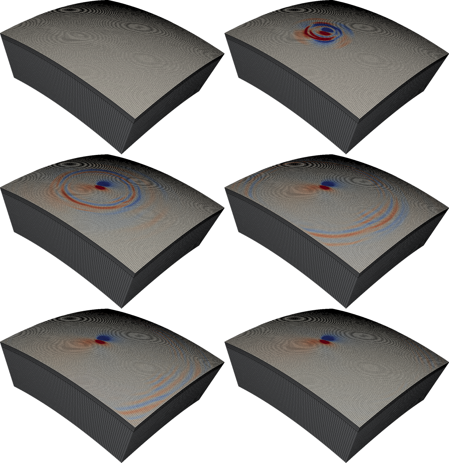
Below is a simulation of the displacement field generated by a tectonic earthquake in Alaska. The computational domain is 2000km wide, too large to ignore the Earth's spherical geometry. Note how well the waves are absorbed by the curvilinear PML at the truncation boundaries.
